USD $99.95          (Money Back Guarantee)       Registration key shipped by email

WOW! - Customer support before you buy!

PANCROMA™ Frequently Asked Questions

This page lists some questions that PANCROMA™ users have asked in the past. I listed my answers in order to provide some instant feedback in case you have the same problem. Do not hesitate to contact me directly if you have an issue, whether you are a customer or just trying the software. If you find a bug, try installing the latest version of the software. It this does not help, please report the problem. The fastest way is to email me with a short description of the problem, along with a copy of the dialog text and error messages. I will do my best to correct all such issues with the highest priority. Your satisfaction is my number one concern!

How do I upgrade to the latest PANCROMA™ version?

The latest PANCROMA version is always available from the Downloads page. Simply download the newest version and install. You will not have to re-enter your registration key nor should you even see the registration key input form, unless you are installing on a new computer. It is not necessary to uninstall an old version to install a new one. Before uninstalling the old version, make sure that you are happy with the new one as archived older versions may not be available.

Where can I get Landsat data?

Free Landsat data is available from several sources. Look at the links on the 'Data' page on this website or under the 'Help' menu selection in PANCROMA™.

Which Landsat database is the best?

Each of them have their advantages. The USGS GLOVIS site seems to have the most comprehensive set of Landsat data with dozens of data sets per scene. GLOVIS also archives ETM+, TM and other legacy Landsat data.

GLCF has less Landsat selection but may be a bit more user friendly. USGS Earth Explorer seems to duplicate the GLOVIS data. Canada's GEOGRATIS has only Canadian scenes. These sites may be worth searching if you cannot find what you are looking for on GLOVIS and GLCF.

The sites are confusing. How do I actually download the data?

GLOVIS and GLCF both have tutorials and help files on their sites. Also, there is a GLOVIS tutorial video on the Videos page of this website. Alternatively, flog around for a while and you will learn eventually.

The GLCF site archives two types of Landsat files: .tif and .L1G. Which should I select?

Landsat data can be archived in a variety of formats. Geotiff (.tif) is the most prevalent. GLCF archives a considerable amount of .L1G format data. PANCROMA™ can import either. Don't try to mix data however.

User writes: Where can I download free SPOT data?

The USGS Earth Explorer website archives SPOT color composite data that PANCROMA™ can decompose to the band files. The Canadian GeoBase website offers full SPOT band data for all of Canada. See the 'Free Data' page on this website or the 'Help' menu.

PANCROMA™ seems like a complicated program. How can I best get started?

It is not as complicated as it looks. PANCROMA™ is composed of many utility routines, each of which is straightforward to learn. Few users need all of them. Start by importing and a single band and displaying a grayscale image. (Grayscale is all you can produce from a single image.) Next import three bands (bands 1, 2 and 3 corresponding to blue, green and red channels) and display an RGB (color) 30m resolution image. These are both easy to do. Experiment with the image processing utilities to become familiar with how they work.

The next step is to subset a set of Landsat images. Import bands 1, 2, 3 and the panchromatic band (these have …10, …20, …30 and …80 file suffixes. Create and save a matched set of cropped data. This is essential for learning the pan- sharpening process as trying to iterate complete files is too cumbersome when learning. Use this file set to try pan sharpening. Forget about image processing the first time. Just see if you can create a high resolution (15m) color image.

Then progress to using the image processing utilities to get a better pan sharpened result. Be sure to use the 'Maintain RGB Comparison Image' feature to get the best results.

I tried to display a single band image and all I get is a black screen.

Scroll down and to the right. You are parked on the black image collar. Landsat images are surrounded by a substantial black collar because the satellite path orientation.

There are seven Landsat bands. Which ones do I use?

Each band file corresponds to a different sensor on board Landsat. Bands 1, 2 and 3 (blue, green red) are the most useful for producing images that match the true color of the image. However, the other bands are extremely useful. For example, since blue light is easily scattered by the earth's atmosphere, particularly by water vapor in the atmosphere, band 1 usually produces the murkiest image. Very interesting images can be produced by using bands 3, 4 and 5 instead of 1, 2 and 3. These produce colors that resemble true color but the image is much clearer as a result of these bands "seeing" through atmospheric haze better. They also tend to reveal interesting features of the earth's geology not easily visible in a true color image.

PANCROMA™ will not let me output my processed file in .jpg format. Why not?

Pan sharpened and even panchromatic Landsat files are very large. The JPEG file compression routines in the libraries used by PANCROMA™ must all duplicate the full image data set into a flat (unsigned char) array before starting the compression. PANCROMA™ offers work-arounds like disabling the image display for large files (see the Instruction Manual). Saving your images in PNG format is another alternative as the PNG writer is much more memory efficient than the JPEG writer. PNG files compress to nearly the size of JPEGs and have the advantage of being a lossless compression.

I keep getting an 'Out of Memory' error when subsetting Landsat files.

Most computers should be able to subset an entire set of band and panchromatic files if you uncheck the 'Display Subset Images' check box on the subset Information dialog. The process will take more or less time depending on your computer.

How long will it take to pan sharpen a set of Landsat images?

Pan sharpening a full-size Landsat data set requires more memory than the Microsoft operating systems will allocate to a single process. As a result data must be written to hard disk scratch files, which considerably slows down data access. It will take approximately 850 seconds with a fast computer. At the other end of the spectrum, I was able to successfully pan sharpen a full Landsat data set, save the pan sharpened image in .bmp format, and display the image in Paintshop Pro on my 1.1GHz, 256MB RAM Windows XL laptop. The pan sharpened image was 17,108 by 15,156 pixels and was 759MB in size. PANCROMA™ version was 1.12. It took about 3 hours to process the data on this machine.

User writes: I got an 'Out of system Resources' message when saving my pan sharpened image.

A common problem is memory resident utilities such as virus shields and the like that use a lot of RAM. Try disabling these during PANCROMA™ runs. You can see how much memory is used by such utilities by calling the Windows Task Manager and examining your program resources.

User writes: The subsetting option should be explained before the pan sharpening instructions so that if the pan sharpening of the original image fails the person will immediately know what option is available. I had to search around your instructions to find this myself.

Good point. Most users may not need the full sized pan sharpened image any way. I added a 'Getting Started' topic up front in the Instruction Manual that highlights this.

The grassy vegetation areas of my pan sharpened image have a blue cast to them. What is wrong?

The HSI transformation and inverse transform used by PANCROMA™ is nearly perfect. Test images transformed from the RGB band files to their corresponding HSI bands, expanded, interpolated and then transformed back to RGB match the input files almost exactly. Color distortion is a result of the characteristics of the panchromatic band that is substituted for the Intensity band before the reverses transformation is performed during pan sharpening. The panchromatic band represents radiated light in wavelengths of 0.52 to 0.90 microns. This includes the visible green, red and near IR bands. When it is back-substituted in place of the Intensity band, the colors in the resulting pan sharpened image do not exactly match those of the RGB color composite image constructed from the low-resolution input files. This is because the panchromatic band does not exactly match the Intensity band computed from the input RGB bands. The problem cannot be avoided but it can be corrected. In some cases the correction is nearly perfect with little extra effort. In other cases minor distortions remain even after extensive automatic and manual image processing efforts.

The most useful correction to this problem is to correct distortions caused by the panchromatic image spectral sensitivity using the NIR band 4 data and the XIONG or AJISANE algorithms. These techniques can greatly improve the result, often eliminating the problem completely. Histogram matching, performed automatically by PANCROMA™ (upon command) adjusts the grayscale level of each pixel in the panchromatic band to more closely match the corresponding pixel in the computed intensity band. This can also result in a pan sharpened image with less color distortion. PANCROMA™ offers two histogram match methods: linear and non-linear. In general the non-linear method is superior. A non-linear histogram match is performed by PANCROMA™ as the default condition.

I pan sharpened my image using non-linear histogram matching and the forested regions of my image are still blue. What should I do?

You can use the ENHG Enhanced Green color adjustment for stubborn images. This technique uses the NIR band in addition to the red, green and blue bands to identify and correct the areas of your image covered by vegetation. See the Instruction Manual for more information.

I downloaded the extra NIR band and used the ENHG automatic method. The vegetation is now green but it does not look natural.

The XIONG algorithm is actually the best for correcting the spectral distortion described above. To use it, load five bands (Blue, Green, Red, panchromatic and NIR) and then select 'Pan Sharpening' | 'HSI Transform' | 'XIONG Five File (Automatic Method)'.

I went step by step through Video 7 with the same image set and got a different output (very dark areas).

The reason that you did not get the same result is that I added histogram matching since I recorded the video. To get the same result, disable histogram matching. Check the 'Activate Image Processing Routines' check box on the main form before pan sharpening. When the image processing box appears, click on the 'No Histogram Adjust' radio button. Then select 'Process Image' This will cause the image to be pan sharpened without histogram matching and you will get the same result that I did.

The black areas are an artifact of the histogram matching algorithm. Certain pixel values will cascade all the way down to zero during the match of the two cumulative histograms. The matching algorithm still needs some help to overcome this issue which occurs only for some images under some conditions. The 'remove highlights' check box invokes an algorithm to solve a similar problem on the high end of the histogram i.e. unwanted cascading toward pixel value 255. I was also able to get rid of the black spots by unchecking the 'clip tails' checkbox but I was not happy with the color result either however. I got the optimum result by using the linear histogram matching instead of non linear matching. Use the radio buttons mentioned above to select this.

Histogram matching can be a very powerful aid but it can also cause unwanted side effects. Settings that work well for one image may not work for another. The defaults I set up work well for most Landsat pan sharpening tasks. SPOT images may benefit from different settings.

Where can I get more information about pan sharpening and PANCROMA?

I periodically publish articles on new utilities and special techniques at www.TERRAINMAP.com

Why does Digital Globe offer their data sets in both 8-bit and 11-bit format? How can I pan sharpen the 11-bit data?

To answer the question it is important to distinguish between dynamic range and bit depth. The dynamic range refers to the capabilities of the sensor while the bit depth refers to the capabilities of the display system. In order to pan sharpen or display data with a higher dynamic range the 11 bits must be rationalized into 8. PANCROMA™ offers two ways to do this. See the Instruction Manual for more information.

I have higher resolution grayscale imagery than the 15m Landsat panchromatic band. Can I use it to pan sharpen Landsat band data?

You can pan sharpen Landsat RGB data with any high resolution imagery as long as the following conditions are met:

• The high resolution image must be an even 2X, 3X or 4X multiple of the Landsat band resolution to pan sharpen using PANCROMA.
• The four images must be perfectly co registered

If you discover a useful source of high resolution imagery with another multiple of Landsat band data let me know and I can add the capability to handle it to PANCROMA™.

I tried to open my GeoTiff format data files but PANCROMA™ does not read them. What is the problem?

PANCROMA cannot currently read compressed or tiled TIFF format. You can tell if the file is compressed by looking at the compression tag value reported to the echo screen. If it is other than '1' then the file is compressed. PANCROMA™ reads the more common stripped TIFF format but cannot currently read tiled format. Native Landsat and SPOT data is always archived in uncompressed stripped format. However, some GIS applications will save in compressed or tiled format. So if you are preprocessing in another application and then importing to PANCROMA™, you may encounter this problem.

A possible remedy is to adjust the 'save' settings on your GIS export application if possible. Alternatively, you can save in JPEG, BMP or PNG format. You will of course lose any embedded georeferenceing information if you save in other than GeoTiff format.

How large of a data set can I pan sharpen with PANCROMA™?

The program was designed to process Landsat data sets. Landsat multispectral bands are typically around 8000 by 8000 pixels while the panchromatic band is double this, around 16,000 by 16,000 pixels. It is possible to process larger data sets. The maximum size will depend on current program architecture, your hardware configuration, and the limitations imposed by the Windows 32-bit operating system that many will use. A panchromatic band size of 20,000 by 20,000 pixels may represent the practical upper limit at present. Larger data sets may result in 'out of memory' error messages followed by abrupt termination of the program.

PANCROMA™ has two special utilities designed to handle huge files. The 'Display One File' utility is set up to read band data directly from disk to a display color model, with no internal array. This will allow displaying a single grayscale band file of relatively large size. The 'Subset One Band' is designed the same way, allowing subsetting of single bands of similarly large size. As a result you can typically subset extremely large data sets down to a size within PANCROMA™'s processing capabilities.

I saved my georeferenced file using ArcGis, but I cannot open it using PANCROMA™. What is the problem?

[Note: this answer is OBE. PANCROMA™ can now read GeoTiff tiled images]. ESRI ArcGis exports Geotiff in tiled format. Tiled format is much less common than the stripped format that Landsat and SPOT data use. PANCROMA™ cannot read tiled images at the moment. I plan to add this capability as an upgrade soon. Until then you might try the following procedure, which was reported by Luke Pinner on the ESRI Support Center website for switching output from tiled to stripped:

Open C:\Program Files\Common Files\ESRI\Raster\defaults\tiff.pdf (note: file is NOT Adobe PDF format, it is ascii, open in a text editor) and change the following line:

create_tiled_images("Create Tiled Images"): "true" "Make newly-created TIFF images tiled

instead of

stripped" boolean "true" "false"; TO

create_tiled_images("Create Tiled Images"): "false" "Make newly-created TIFF images tiled instead of stripped" boolean "true" "false";

Loooots of other TIFF options in there including compression. Thanks to Matt Wilkie for pointing this out recently in an ESRI-L SUM.

Note:The file is loaded on startup, so exit and restart all ArcGIS programs before testing... And don't forget to make a BACKUP!!!

I saved a GeoTiff file using Global Mapper but PANCROMA™ would not open it. What is the problem?

Global Mapper saves GeoTiff files in compressed format, which PANCROMA™ is not able to handle at the moment. To fix this, change the default 'packbits' compression to 'no compression' in the Global Mapper GeoTiff export options dialog box before saving the file.

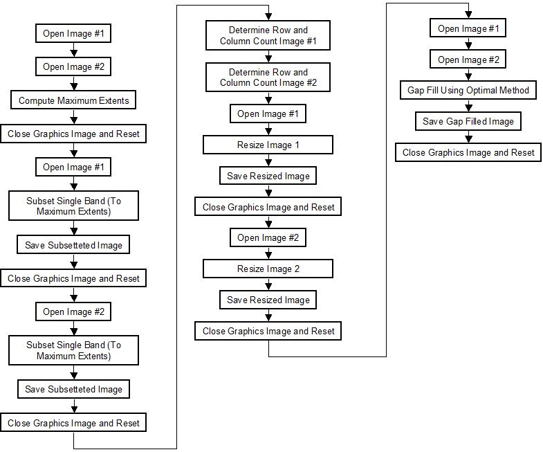
I tried to use the three-file cloud mask utility on my Landsat scene but I keep getting an error message stating 'Unexpected Row and Column Sizes'

The cloud mask utility, like most PANCROMA™ multi-file utilities requires exactly matched row and column input files. In the case of cloud masking, the Landsat TIR bands are approximately half the row and column count of the band files, but not always exactly. Sometimes they are off by one row or column. Before cloud masking, you must resize the files so that they have the required 2X row and column ratios before masking. You can resize downward use the PANCROMA™ 'Preprocess' | 'Resize Images' utility. See the Instruction Manual Section 31 for more information.

After loading the image in PANCROMA™, some of the menus are still disabled, why?

Certain menu selections will initially be disabled. They will become enabled as you open input files and process them. For example if you open a single band file, then all the menu selections appropriate to processing a single file will become enabled, and all those that require two or more input bands will be disabled. When you open a second band file, the menu selections appropriate for processing a single file will become disabled and those that require two input files will become enabled, etc. When you are done processing a data set, select 'Close Graphics Windows and Reset' to start over again processing a new data set.

I'm trying to do a standard 3-band combination using Bands 3, 2, and 1 of a Landsat scene. I'm opening them up in PANCROMA™ in the order I want to combine them (in B,G, R order) and everything appears fine until I try to do the band combination. Then, I get two warnings 1) "The utility wants bands input in this order: blue, green. red" and then crashes with 2) "Unexpected row and column sizes. check your input sizes" I can display each band individually with no problems.

It appears that the problem is that all three of your input files are not exactly the same size, i.e. they do not all three contain the same number of bytes. PANCROMA has three levels of file sentinels. The first level checks to see if all three input files are the same size as mentioned above. The second level checks that the file characteristics are correct, i.e. that the file is uncompressed, the bits per sample is 8, the planar configuration is either 1 or 2, etc. The third level checks to make sure if the row and column counts all match up. The reason I do all this checking is that if the files are not consistent, it can cause an untrapped error. These are usually caught by the operating system but at best they would cause PANCROMA™ to crash by over writing an array or some similar misbehavior. PANCROMA™ apparently feels that the byte count in all three files do not exactly match and is declining to process them as a precaution. I have never seen such a mismatch with Landsat files downloaded directly from any archive source. However, if one band file is processed by another application, it is possible that the application is writing to the GeoTiff ASCII fields and causing one of the bands to be larger or smaller by a few bytes.

I uploaded PANCROMA™ version 4.95 tonight that will report the three file sizes if the sentinel is tripped. I also corrected the dialog box error message that reported a row and column size error when the problem is really the file size. One usually causes the other but not always.

If you would not mind downloading the new version and letting me know if the dialog screen reads something like:

File Checksum Error. The input files are not consistent .tif Landsat files. band1FileSize is: 169926
band2FileSize is: 169926
band3FileSize is: 169928 <--- Note different file size

Update: PANCROMA™ version 4.99 has a switch to disable the file size verification sentinal.

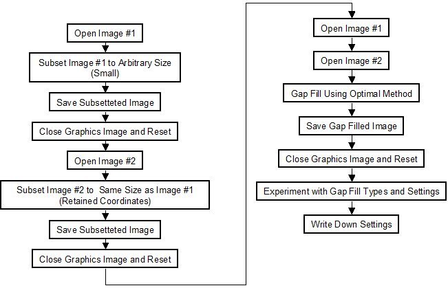
I am trying to subset two Landsat scenes for gap filling. I subsetted the first set OK. When I loaded the second set and entered the coordinate data I got an error message. What went wrong?

When you process the second set, just check the 'Select by Coordinates' radio button. Do not enter any values into the text boxes, as the correct values from the previous scene have been automatically entered into the text boxes. After you have checked the radio button, select 'Enter' and the second set will be subsetted to the same corner coordinates as the first set.

I was wondering if you could offer some advice regarding some pre-processing issues I am having. I am trying to gap fill a Landsat 7 ETM SLC-off thermal image. I have Landsat 7 slc-on thermal image to fill the SLC-off image. I understand that the images need to be subsetted before the gap filling can be done. Here is where I am having difficulty. Is there a step by step procedure that you could recommend for subsetting?? Would you recommend the rubber band method or entering the exact x,y coordinates?

You do not have to subset images to gap fill if the following conditions are met between the two images:

1) The corner UTM coordinates must match exactly
2) The row and column counts must match exactly

These two conditions imply that the xScale and yScale values are the same also.

Since this is very rarely the case with two Landsat scenes the images have to be slightly cropped and adjusted to meet the above conditions. There are several ways to accomplish this. See Section 25 of the Instruction Manual for information.

For just filling two thermal bands you can use this manual method:

Use the 'Compute Common Extents' utility to determine the UTM coordinates of the overlap area by opening the two files and then selecting 'Band Combination' | 'Subset Images' | 'Compute Maximum Common Extents'.. This utility *only* computes the coordinates of the overlap region and then copies them to the coordinate text boxes in the Subset Data Entry form. You need to follow that operation by the following operation (without exiting the program):

1) Selecting 'Close Graphics Coordinates and Reset'. This closes both files but retains the coordinate information in the text boxes.
2) Then select 'File' | 'Open' and re-open one of your two files.
3) Select 'Band Combination' | 'Subset Images' | 'Subset One Band'. When the Subset Data Entry form becomes visible you should see the corner coordinates already entered. I attached a picture of what the form should look like at this point.
4) Select the 'Select by Coordinates' radio button.
5) When you select 'Enter' the subset will be computed and displayed.

Now select 'Close Graphics Window and Reset. Repeat steps (2) through (5) for the second image. The UTM coordinates will persist in the text boxes for as many images as you wish to subset.

I just updated Section 17 of the Instruction Manual to include these instructions. (You may have to download the latest version).

Alternatively, all this can be done automatically by using the procedure described in Section 60 of the manual. This utility wants six input files, three gapped and three ungapped as it was designed to preprocess two sets of three multispectral band files. However you can just load three copies of each of the two thermal bands and it will work just as well. There is a video on the website that demonstrates this utility.

Regarding the last part of your question. If you want to gap fill the entire Landsat scene, use the 'Compute Maximum Common Extents' utility. If you are interested in a small subset, you can use any of the three methods for selection of your area of interest. Your case is a bit special as you are only interested in the two thermal bands. In that case you will have to subset a single band twice, using whatever method you want for the first image and then check the Coordinates radio button for the second so that the retained coordinates are used to subset the second image.

In other words, no matter what you do, the coordinates persist in the text boxes so that you can use them to subset subsequent images.

Watch one of the videos and it will be a lot clearer than my narrative.

Thanks for the advises and it works smoothly! But now, another problem comes up when I tried to gap-fill the 2 registered scenes. The gap-filling function is workable, however, the resulted image have some obvious banding strip. I tried Hayes and then Teras method referring to the manual, got no significant improvement. ( using default setting values) And the gap-filled images are attached for your reference. Please advise, thanks very much!!!

Congratulations on getting this far.

The quality of the gap filling is MOST dependent on the quality of the images that you are trying to match. A good rule of thumb is that if you get poor results with the simple Transfer method, it will be a struggle to get a good match no matter what you do. I believe this is the problem in the RGB image of San Francisco for example. The color tones match well, but it looks like the fill image is hazy and as a result you are losing features in the fill areas. This can be seen in the stripe that crosses the Golden Gate bridge. You might be able to fix this by using the PANCROMA™ Haze Reduction utilities on the fill image, or else select a better image. I attached two sets of examples that illustrate good and bad band selection choices.

Here are a few other ideas:

1) The most important factor is atmospheric conditions. If one of the images was acquired under clear conditions and the other under hazy conditions, the results will not be so good.
2) Next is season. Reflectances from vegetation, the state of tilled fields, etc. will vary drastically between seasons. Try to get images acquired at least in the same season, and as close in calendar dates as possible.
3) Try to get zero cloud cover images if available.
4) Consider using two (or more) post-2003 gapped images rather than a pre-2003 and post-2003 clean and gapped image. This will allow a wider selection of images from which to choose and will get the acquisition dates closer together.

I believe that the USGS considers these four factors very carefully in selecting candidate images for its gap filling work.

Regarding software settings. Here are some ideas

1) Most Important - create small test subset images for quick experimentation. Once you are satisfied with the results on the subset, apply the same settings to the full scene.
2) Look at the details of your image to determine the cause of residual striping. Is it poor color tone match or resolution mismatch?
3) Experiment with the settings on the Gap Fill Data Form for the Hayes and TERAS methods. The significance of the settings is explained in the Instruction Manual. These will have some impact but no setting can compensate for a bad Scene selection. There is some tradeoff between tone quality and resolution for the Search Extents setting for example.
4) Consider preprocessing one or both images before gap filling. The Haze Reduction, Surface Reflectance and TOA reflectance utilities are designed to improve image fidelity by eliminating effects caused by the atmosphere, the difference in solar angle at time of acquisition, distance from the Sun, and other factors.

We have to fill an SLC-off Panchromatic scene with another SLC-off scene. Remaining area is to be filled with a SLC-on scene. I tried doing as per the manuals but I get stuck at subsetting part. I know there is there is a great deal of helping manuals and videos on your website. Still after going through them I am not able to do it. I would appreciate if you could provide a step by step guide for this specific project.

The subsetting exercise can be done a number of ways but the best way is to use the six file automatic method. The instructions are given in Section 61 in the instruction Manual (Tutorial - Six File Automatic Method) and also shown in the video entitled Automatic Subsetting Six Landsat Files.

To prepare six Landsat files for subsetting you basically open three from the first set and three from the second set and then select Band Combination | Subset Images | Subset Six Bands and then select 'Enter' when the data input box appears. Then save your subsetting images by inputting the base name by selecting File | Save Subset Images | Geotiff. The band 1 matchups will be 'basename'1.tif to 'basename'4.tif; the band 2 match will be 'basename'2.tif to 'basename'5.tif; and the band 3 match will be 'basename'3.tif to 'basename'6.tif;

Of course there must be some overlap area between the two data sets or this process will not work. I posted some example files at my ftp site in a directory with your name on it. The log in info is as follows:

When gap filling additional sets, you should just repeat the six file procedure after gap filling the first set. In this case you will have one set of three (partially) gap filled band files and the third set that you have not used yet. Just repeat the six file subsetting method with these two sets. This can be repeated for as many data sets as necessary.

We were able to fill a subset of the image using Hayes method. I find artifacts like in the attached screenshot. Can you please explain. How do we improve the results?

I recommend taking a look at the Tutorial in the Instruction Manual in Section 69. The workflow that is outlined in that section is relevant to the panchromatic images that you uploaded if you are planning subsequent pan sharpening. The Tutorial is dated as the PANCROMA pan sharpening methods have improved since I wrote it and it is now a lot easier to get balanced color tones without all the effort described in the section.

Keep in mind that it is very difficult to gap fill an entire scene without some areas that turn out less than ideal. Problems can arise from clouds, snow, and differences in TOA reflectance; solar elevation and azimuth; seasonal variations, etc. between the two scenes That being said, here are a few tips to keep in mind.

• Look at the information in the Instruction Manual for each of the gap filling methods. They explain generally how they work and what the settings do.
• For both the Hayes and TERAS methods, the Search Extents often has to be increased to get good results. The Search Extents must be greater than the maximum half-width of the widest gap.
• For the Hayes method, increasing the Comparison Radius is sometimes necessary in order to collect enough pixels for a valid computation. However increasing the Comparison Radius can also cause an unwanted smoothing effect.
• For the TERAS method, the Cloud Saturation Cutoff sometimes needs to be increased in order to avoid ignoring highly reflective image pixels caused by snow or salt pans.

When I gap filled your images, I had to increase the Search Extents to at least 22 because the gaps were wide. Generally the greater the Search Extents the better the quality of the gap fill but the longer it takes to process the image.

The Hayes method was troubled by dark shadows caused by mountain peaks. PANCROMA™ could not find pixel matches outside the gap strips sometimes so it just transferred pixels in from the ungapped image. This caused some dark anomalies in the image.

When I used the TERAS method I had to increase the Cloud Saturation Cutoff in order to avoid ignoring pixels in the salt flats. I increased it all the way to 255 since there were no clouds in the image. I uploaded my results for each of the three methods to your folder.

I'm looking at ASTER data and have downloaded the files, but now the process of converting the .hdf file to geotiff. I have both Multispec and HEG loaded and not having much success with either. You mention you have detailed instructions for this process, could I get a copy?

The procedure for converting ASTER HDF data with MultiSpec is as follows: Open MultiSpec. Select 'File' | 'Open Image' and open the ASTER HDF format file. All of the ASTER bands are bundled in the single HDF compressed file. A Dialog box will become available. At the bottom of the dialog box there is a drop down menu entitled HDF Data Set. This is where you can select the ASTER band that you want to display. Select 'OK'. A second dialog box will become available. In the 'Type' drop down box select 'One Channel Grayscale'. (If you do not you will get an RGB image. I have not yet figured out how you control which bands go into the RGB composite. The band numbers are displayed in the border at the top.)

PANCROMA has a naive GeoTiff reader that assumes 'North is Up'. It looks at the Northwest corner coordinate and then uses the Xscale and Yscale GeoTiff data to display the image. ASTER band images are aligned with the swath, which is about 10 degrees off true North. You must instruct MultiSpec to convert the image in 'North is Up' format to maintain coordinate integrity. On the MultiSpec menu select 'Processor' | 'Reformat' | 'Rectify Image' . Check the 'Translate, Scale and/or Rotate' radio button and then check the 'Use image orientation angle' check box. The saved image will be reprojected in 'North is Up' orientation. (If you don't care about the coordinates you can skip this step.)

Select File | Save Image to GeoTiff As. Save the file. Repeat for as many of the ASTER bands that you want to convert. There are variations on this procedure that will work. For example you can save three bands as a composite image and decompose them to the band files in PANCROMA™.

I just want to understand more about the gap-fill process using Hayes method. Can you just describe briefly what the software is doing in the background when it's doing Histogram matching and filling the gaps? All I know is that it's doing Histogram matching between reference and adjust image but I don't really understand fully what is going on in the background.

The Hayes method does not use a histogram match approach. The Transfer method does use a global histogram match. The problem with global adjustments is that each adjusted pixel is affected by every other pixel in the image. This produces a generally OK result everywhere but an optimal result virtually nowhere.

The Hayes method is a local optimization method. A so-called sliding window size is set by the user. Only pixels within the boundaries of the sliding window influence the adjusted pixel. After computing the new value for one pixel, the window indexes over one pixel and the optimization is repeated. This is done for every pixel in the image, or more correctly for every pixel that falls within a gap in the image. This is why local optimization methods take longer. There are as many computations as there are pixels within the gaps, which can be a lot. However the result is generally better because only pixels proximal to the target are considered. The TERAS algorithm uses a different local optimization algorithm.

The exact nature of the computation that goes on inside the sliding window is proprietary. However as the Instruction Manual states, comparisons are made between a target pixel in the no gap image, surrounding pixels in the no gap image and corresponding pixels in the gapped image, and a value for the missing pixel is computed

Another question, Can I get negative value when calculating TOA reflectance? Does it make sense?

It is definitely common to see (usually slightly) negative reflectances when converting Landsat DNs using the proscribed conversion equations, and they probably appear for the other multispectral sensors as well. I guess these result from non ideal sensor responses, although I have not seen an explanation from the data providers about this phenomenon. Since a certain percentage of incident light is reflected, and 100% minus that percentage is absorbed, a negative reflectance would mean that more than 100% of the incident light is absorbed, which cannot make physical sense.

PANCROMA™ sets any negative reflectances that result from its computations to zero, assuming that the values are small and are a result of minor sensor problems as stated. I suppose I should at least provide information about any negative values so that the user can decide whether to discard the band image and use another. Maybe in the next release.

I have been trying a couple things on trial mode and I cannot get my landsat images to appear in the display. The screen appears black and I cannot zoom. Also when I walked through a GAP fill tutorial, some of the menus structures and names have changed so it was very confusing to go through. I just read that I cannot save until I get a registration copy which solved one issue I was having. But I am finding it very hard to follow the instructions in the tutorials. Could you possible provide some insight on why my images are appearing completely black and not in the grayscale or color?

The first problem: all black screen Landsat image. I believe that this must be because your image is centered on the upper left corner by default on the black collar of the Landsat image. Because the Landsat paths are not aligned north/south, the rectangular images are rotated to the right, yielding a black collar around the image. You should see the image if you grab the slider bars and move the image center to the display center. All PANCROMA™ images are displayed at full scale by default. You should be able to zoom out once you center the image. If this is not the problem please let me know.

The second problem: gap filling. You are correct about the menu selections not agreeing with the videos as I reorganized the menu selections a few months ago but did not re produce all the videos. This weekend I fixed the first video that you need: Automatic Subsetting Six Landsat Files. I created a second one entitled 'Gap Fill Transfer Method'. These are videos 15 and 16 on the Videos page on the website and will show you how to do it. Note that gap filling using the Hayes or TERAS methods is exactly the same as the Transfer, except for the menu selections of course.

Can I load five bands in the order: band1; band2; band3; band4; band5 and band7 of Land sat, for subsetting without the panchromatic band and the results would be the same sequent? And no changes in the data structure?

You can subset five multispectral bands by selecting the 'Subset Five Bands' menu selection. This selection will detect whether the fourth input file is a multispectral band or the panchromatic band and will subset accordingly and the fourth file entered will be OK no changes to its data structure.

When you save (as GeoTiff for example) and specify a base file name (baseFile for example) the five subsetted multispectral bands will be saved as baseFileband1.tif; baseFileband2.tif, etc. in the same order that they were input.

You are correct about the PANCROMA file naming convention. When you subset four multispectral bands, the output files are numbered 1, 2, 3 and 5, anticipating one possible case where the visible plus NIR bands are being subsetted. However the program always numbers the output files in ascending order consistent with the way that they were input. You can just rename the files to the right band numbers afterwards.

You actually listed six input bands. You cannot directly subset six multispectral bands in a single operation. However you can subset five multispectral bands as described above. PANCROMA will retain the corner coordinates when you do so. If you want to subset a sixth multispectral band, just select 'Close Graphics Window and Reset' (not Exit) and then open the sixth multispectral band (band 7 in your example). Now select 'Subset One Band' | 8 or 16 Bit to 8 Bit Band File'. You can select by pixels or UTM coordinates using the radio button. Accept the coordinates that are in the text boxes (do not click on the image!) and select 'Enter'. The sixth file will be subsetted to the same coordinates as the previous five. Using this feature, you can subset an arbitrary number of multispectral bands using the one file, three file, four file or five file methods.

You have mentioned in the guide manual!! IMPORTANT NOTE: You must open the files in the specified order or unexpected color tones will result.

This just means that to get a true color image, you must input the visible blue band first, the green band second, and the red band third, otherwise you will generate a false color image.

When I open Landsat 8 scenes, PANCRMA™ reads the projection perfeclty, but when you export an RBG image its changes the projection from South to North hemisphere. Like in Paraguay, we are in two UTM zones, Z: 20 S and Z: 21 S. But pancroma exports geotiff at Z: 20 N and Z21N.

This one was pretty embarrassing for me. I originally thought that the problem the user was having resulted from the Projected CS Type Code being wrong. The USGS for some reason lists the CS Code is 326 instead of the correct 327 indicating the wrong hemisphere.

It turned out that the problem was a build error for the PANCROMA version 5.97.77. The build error led to an access violation in the data structure used to store the UTM coordinates. This in turn caused the upper left UTM coordinate to be reported as (0, 1) instead of the correct values. I was able to correct the problem by rebuilding and posting an updated .exe file.

I work at the moment with Landsat 8 images and I have a few questions. If I choose the preprocessing methods "compute Radiometric corrections > Landsat 8 TAO Reflectance", then DN is converted to Reflectance? Now, if I make a RGB composit with the Reflectance Imagnes, then I see later color values ??0-255. What I do not understand? Then the second question: I would like to make a DEM-based haze reduction. Is that possible with Landsat 8 pictures too? And generally, how should I best proceed: First, a haze optimized transformation, then a DEM based Haze correction, and then a Landsat 8 TAO Reflectance transformation?

The main purpose of reflectance data is to compensate for solar angle and solar distance effects and also gain and bias differences among band sensors. Satellite reflectance values typically range between 0.0 and 1.0 (although they can be higher). Your Landsat 8 Reflectance image has values between 0-255 because it is scaled by the amount specified on the TOA Reflectance Data Form, Graphics Image Scale Factor. The default value is 500, but you can set it to 1.0 to plot the actual reflectance values. Of course this will produce an all black image. You can also write the raw reflectance values to a binary IEEE32 float file by checking the appropriate box on the TOA Reflectance Data Form. The scaled reflectance data can be saved in either 8 bit (default) or 16-bit format (by checking the box on the TOA Reflectance Data Form.

Theoretically reflectance based images from different scenes, all with the same scale factor should have matched brightness tones. This can help when creating mosaics or otherwise comparing data from different scenes. Except for atmospheric effects.

Images can be further improved by reducing these effects by correction algorithms such as haze reduction. I advocate correcting image data from DNs to TOA reflectance first, then approximating surface reflectance (the Holy Grail of satellite image processing) by applying haze reduction. I usually select a single haze reduction algorithm, but you can apply as many as you wish. None of the PANCROMA algorithms are based on rigorous atmospheric physics for reasons that I explain in some of my White Papers. As a result, their application requires some judgment.

Keep in mind that any atmospheric correction is just an approximation, some approximations being better than others.

We have started doing 'Crop Growth Monitoring' from recent Landsat-8 images and have been creating a database of files to see 'How it Was' becomes 'How it Is' at harvest. Many of our crops are sugarcane - often grown in 50 ha (or so) centre pivots. When we have applied our analyses to the Pan-Sharpened output from PANCROMA - it appears that some band combinations are consistently 'less sharp' than the basic 234 (natural colour) images.

While you are looking into the preferential pan-sharpening of bands - perhaps you can also comment on how the perfectly 'deep blue' of a 4-5-6-combo river or lake gets washed out to a 'pale-blue' to 'grey' when the image is pan-sharpened ?? see attached. In the process, some of the details (like islands in the river) get washed out and lost in the new grey-blue replacement.

I believe that both issues are related to aspects of the HSI pan sharpening algorithm. The basic HSI transform method transforms the 30m RGB bands (in a true color image) to their corresponding Hue, Saturation and Intensity bands. The Intensity band is discarded. The Hue and Saturation bands are expanded so that they match the resolution of the panchromatic band and then interpolated to fill in the missing pixels. Then the panchromatic band is substituted for the Intensity band, and the three are reverse transformed back to RGB color space. Other methods use different color space transforms.

I believe the "jaggies" effect around the irrigation circles are related to interpolation. Interpolation in general is an evil thing, but it is often the best we have to create data from nothing. Interpolation schemes infer missing data from the surrounding pixels. This can work very well when the surrounding pixels are similar to the missing pixels. However if they are not, the computed pixel intensity may not be so good. I believe this is what is happening around the crop circles. There is an abrupt discontinuity in pixel intensities, which creates edge effects related to "borrowing" pixel intensity data from unlike pixels. The effect dissipates rapidly as you move away from the edge.

I ran some experiments using different interpolation methods and iterations and was able to mitigate this somewhat. My example images are attached. The Iterative method with a Laplacian initial solution should yield the smoothest edges. The Iterative method requires a lot of storage and will cause an out of memory error for full Landsat scenes but can be used for subsets. The Laplacian alone did not do so bad.

Regarding the color washing: See the algorithm description above. The bands get transformed, one gets thrown away and a different one substituted. Color fidelity is always a problem with pan sharpening. In your case, it looks like you have processed the RGB bands before pan sharpening, as rivers are not naturally that color. Substituting the panchromatic band should tend to push the colors back toward the tones of the unprocessed multispectral bands. The ELIN processor may help fight that effect. I might be able to provide more advice if you gave me more information regarding the RGB band files.

The PANCROMA routines work well for about 90% of all Landsat-8 sharpening work. This discussion outlines a recurring problem with some band combinations, which tend to result in a 'saturated' pan sharpened image, with heavy tones covering large areas and a semi, or total loss of clarity in others.

I ran some tests on your Landsat scenes. I could not produce the same dark artifacts as you observed but they looked familiar. I believe that they are an unwanted side effect of the default PANCROMA nonlinear histogram matching algorithm. Attached are the results of my tests.

• The first image is an RGB color composite image from bands 4, 5 and 6.
• The second image bands 4, 5 and 6 pan sharpened with band 8. Note un-natural ocean coloring near coast.
• The third image is a subset, pan sharpened as above. Same ocean coloring issue.
• The fourth image is the same subset, pan sharpened with histogram matching switched "off".
• The fifth image is the same subset, pan sharpened with linear histogram matching selected.